Journées I2E

Policy evaluation using Transformer-based medical pathway embeddings

Meilame Tayebjee

10 June 2026

Table of contents

• 1 Introduction
  • About me
  • Broader view of the Graph4Health ANR
• 2 Transformer-based models for medical pathway embedding
  • Setting
  • Objectives
  • Model
  • Pre-training
  • Overview
  • Validating the model
• 3 Use Case: Off-Policy Evaluation
  • Markov Decision Processes and Off-Policy Evaluation
  • In our case
  • Doubly robust evaluation
• 4 Avenues of work
  • Future work
• References

1 Introduction

About me

• Graduated from HEC (19-24), X (X20), ENSAE and MVA (administrateur de l’Insee, 2024)
• Currently, since sept. 2024:
  • Data Scientist at Insee’s AI & Data Science Innovation Lab (MLOps, agentic workflows and deep learning use cases: NLP, ML/DL for econometrics, satellite imagery)
  • PhD in CS Candidate (part-time) - supervised by G. Lecué (Crest) and G. Varoquaux (Inria)

Broader view of the Graph4Health ANR

• The general objective is to
  • infer the impact of the healthcare supply (and its geographic distribution) on health outcomes
    • using classic econometric tools
    • using deep learning methods
  • study policies that contribute to the efficiency of the French healthcare system
• 11 years of exhaustive SNDS
  • 70M patients
  • consultations, procedures, hospitalizations, medications, deaths etc.

2 Transformer-based models for medical pathway embedding

Setting

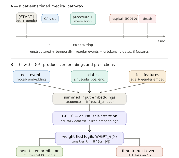
Dataset of medical pathways: For i = 1, \dots, n, X_i \coloneqq (e_i, t_i, f_i), where:

• e_i \in \mathbb{R}^{cs} are the tokenized events, containing integers between 0 and the vocabulary size \lvert \mathcal{V} \rvert
• t_i \in \mathbb{R}^{cs} is the temporal vector, containing the dates
• f_i \in \mathbb{R}^{2} corresponds to the patient general features, (e.g. age and gender)

Tokenization

• Consultations: 83 tokens (specialties, e.g. general practitioner, cardiologist, etc.)
• Procedures: 936 tokens (CCAM codes)
• Medications: 704 tokens (ATC codes)
• Hospitalization entries: 3,275 tokens (ICD10 codes)
• Hospitalization exits: 1,110 tokens (DRG codes)
• Emergency entry: 1 token
• Death: 1 token
• Long-term disease (ALD): 1,110 tokens (ICD10 codes) + 1 token for “no long-term disease”
• Special tokens: [PAD], age, gender, “history token”…

• These pathways are:

  • unstructured (just as in NLP)
  • temporally irregular (not like NLP!)

• To feed downstream estimators, we need to represent those pathways as vectors (embeddings)

Objectives

• Having a time-aware Transformers (\neq NLP) with a lot of simultaneous events
  • Need to design an adapted loss function
• Keeping in mind policy evaluation
  • We want to be able to efficiently compute the embedding of the pathway at any time (the trajectory of the patient)
  • Focus on decoder-only Transformers (GPT-like)

Model

• Embedding matrices of size \mathbb{R}^{\lvert \mathcal{V} \rvert, d_{embed}} (vocab), \mathbb{R}^{2, d_{embed}} (gender) and \mathbb{R}^{8, d_{embed}} (age class)
  • We use t_i to have a time-aware positional encoding using a sinusoidal encoding
  • A symbolic [START] token, composed of the summed embeddings of age and gender.
• Causal self-attention layers so that the Transformer-based model outputs causally contextualized embeddings: GPT_{\theta}(X_i) \in \mathbb{R}^{cs, d_{embed}}

Pre-training

• We use weight tying to output the logits \in \mathbb{R}^{cs, \lvert \mathcal{V} \rvert}

\text{logits}_{i, c, v} = (W \cdot GPT_{\theta}(X))_{i, c, v}

• Next-Token Prediction: instead of softmax as in Shmatko et al. (2025), we use a multi-label classification loss to better handle co-occurent events:

\text{BCE}_{i, c} \coloneqq - \sum_v y_{i, c, v} \log \frac{\lambda_{i, c, v}}{1 + \lambda_{i, c, v}} + (1-y_{i, c, v}) \log \frac{1}{1 + \lambda_{i, c, v}}

• Time-to-Next-Event Prediction: exactly as in Shmatko et al. (2025):

\text{TTE}_{i, c} \coloneqq - \log(\sum_v \lambda_{i, c, v}) + t^{*} \sum_v \lambda_{i, c, v}

Overview

Validating the model

Scaling law

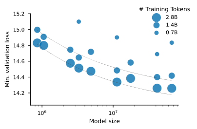
Scaling laws showing the power-law decay (dashed) of validation loss as a function of model parameters and data volume.

We are matching the ~2,000 optimal ratio \frac{\text{\# training tokens}}{\text{\# parameters}} found in Waxler et al. (2025).

Embedding space

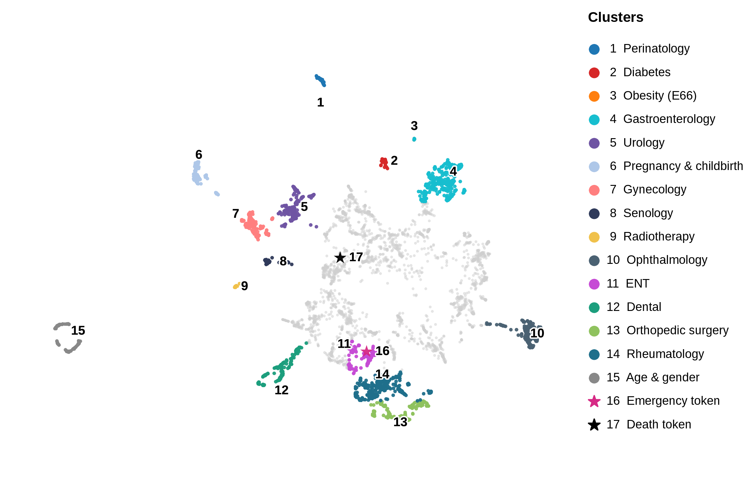
Spatial proximity reflects co-occurrence patterns learned during training on raw medical trajectories, without any explicit clinical labeling. The embedding space spontaneously organizes into interpretable clinical clusters, suggesting the model has learned a coherent representation of medical care.

Time Calibration

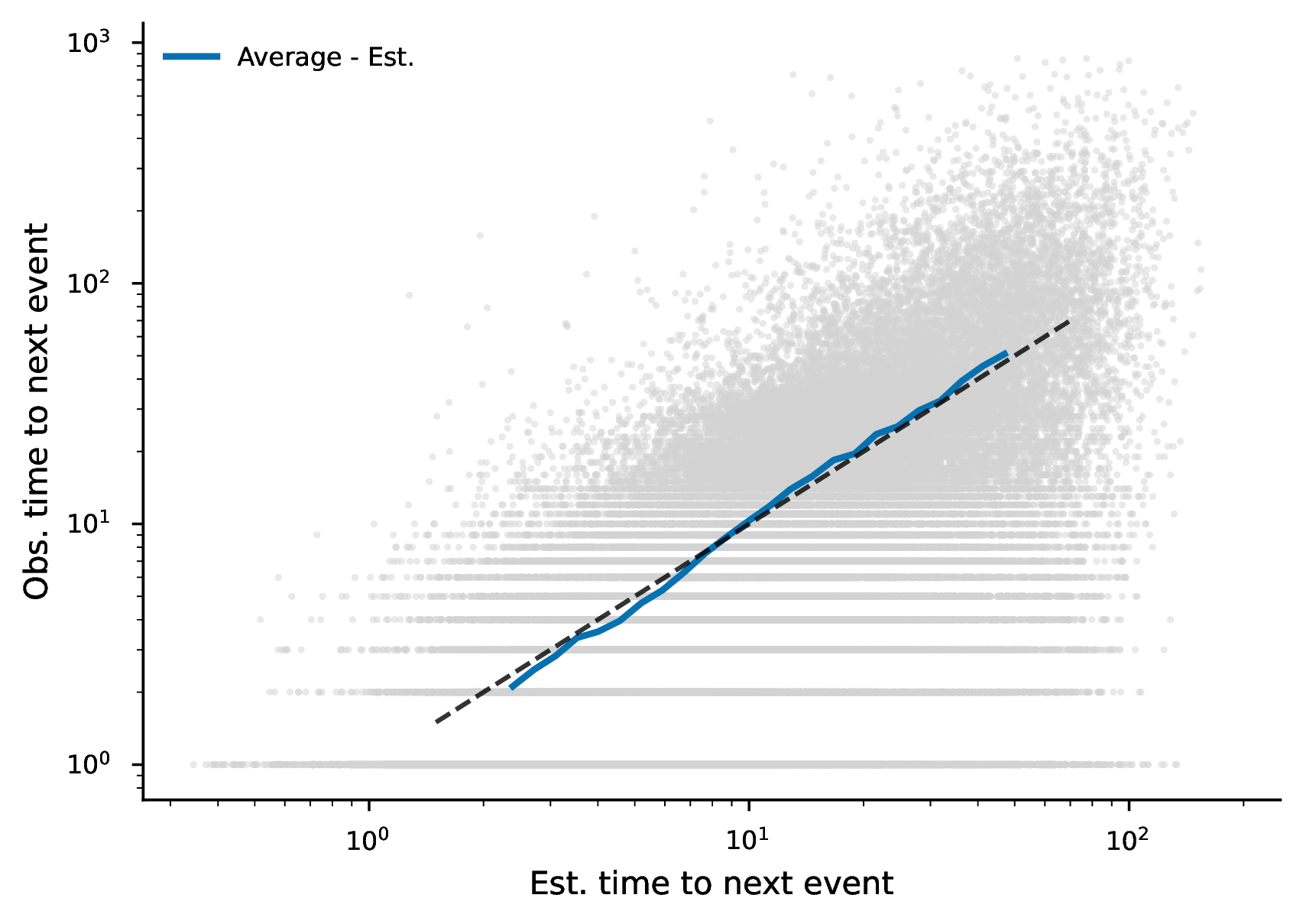
Temporal calibration comparing expected versus observed days to the next medical token; the identity line (dashed) indicates high temporal precision.

Predictive power

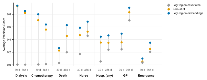
APS across 7 clinical events at 30 and 365-day horizons (n = 100,000 held-out). Each individual’s embedding is sampled at a random time along their trajectory. Blue: logistic probes trained on a separate cohort of 100,000; orange: GPT zero-shot; grey: age/sex baseline.

3 Use Case: Off-Policy Evaluation

Markov Decision Processes and Off-Policy Evaluation

• A Markov Decision Process (MDP) is a tuple (\mathcal{S}, \mathcal{A}, P, P_0, R, \gamma) where:
  • \mathcal{S} is the state space
  • \mathcal{A} is the action space
  • P: \mathcal{S} \times \mathcal{A} \to \Delta(\mathcal{S}) is the transition probability function
  • P_0 \in \Delta(\mathcal{S}) is the initial state distribution
  • R: \mathcal{S} \times \mathcal{A} \to \mathbb{R} is the reward function
  • \gamma \in [0,1] is the discount factor

• A policy \pi: \mathcal{S} \to \Delta(\mathcal{A}) is a mapping from states to distributions over actions (\pi(a|s) is the probability of taking action a in state s under policy \pi).

• A T-step trajectory \tau generated by policy \pi is a sequence of states, actions and rewards: \tau \coloneqq (s_0^i, a_0^i, r_0^i \dots s_{T-1}^i, a_{T-1}^i, r_{T-1}^i, s_T^i) where:

  • s_0^i \sim P_0 is the initial state
  • a_t^i \sim \pi(\cdot | s_t^i) is the action taken at time t
  • s_{t+1}^i \sim P(\cdot | s_t^i, a_t^i) is the next state
  • r_t^i = R(s_t^i, a_t^i) is the reward received at time t

• The return of a trajectory \tau is the discounted sum of rewards: G(\tau) = \sum_{t=0}^{T-1} \gamma^t r_t^i.

• We are interested in the value of a policy \pi, defined as the expected return of trajectories generated by \pi: V^{\pi} = \mathbb{E}_{\tau \sim P^{\pi}}[G(\tau)] where P^{\pi}(\tau) is the distribution of trajectories generated by policy \pi.

• The Off-Policy Evaluation (OPE) problem assumes:
  • We have access to a dataset of T-step trajectories \mathcal{D} = \{\tau^i\}_{i=1}^N generated by an unknown behavioral policy \pi_b: \mathcal{S} \to \Delta(\mathcal{A}).
  • We want to estimate the value V^{\pi_e} of a target policy \pi_e: \mathcal{S} \to \Delta(\mathcal{A}) using only the dataset \mathcal{D}.
• Markov property:

\Pr\{s_{t+1}=s', r_{t+1}=r \mid s_t, a_t\} = \Pr\{s_{t+1}=s', r_{t+1}=r \mid s_t, a_t, r_t, s_{t-1}, a_{t-1}, \ldots, r_1, s_0, a_0\}

The future is conditionally independent of the past given the present state.

In our case

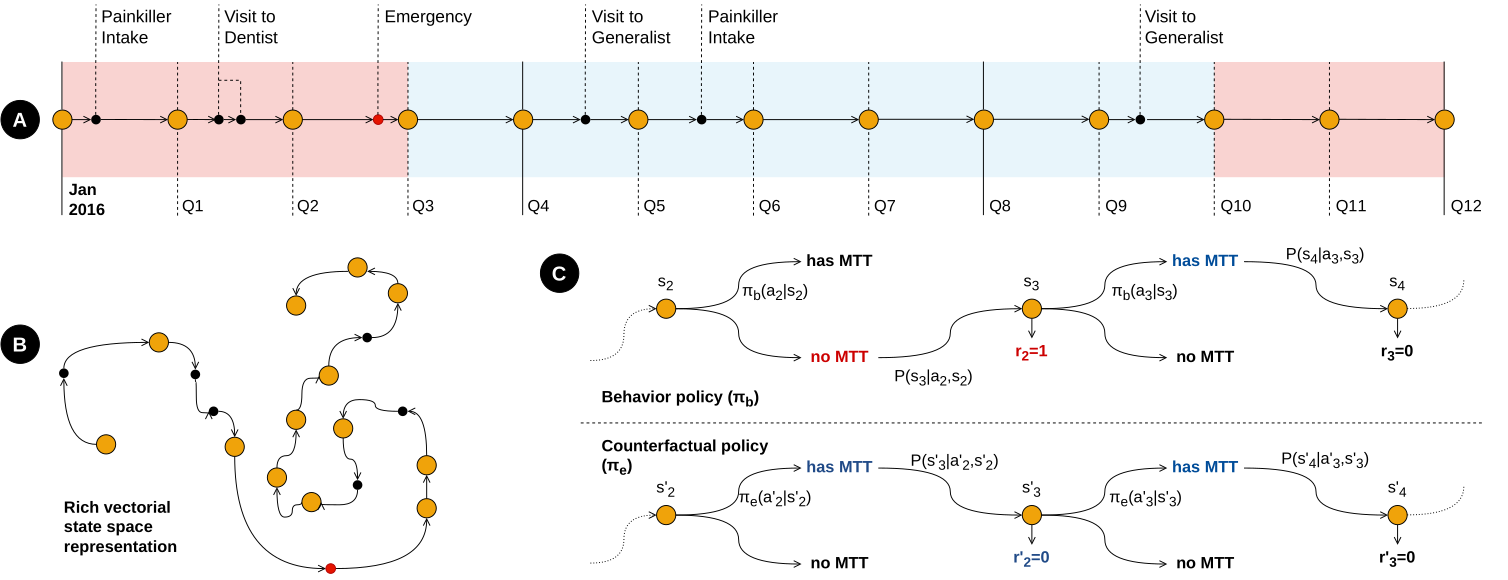
• Dataset: 2 years, discretized into 8 quarters; we define t=0 as the first day of 2017 and T=7 as October 1st, 2018.
• \pi_e(1 | s_t) ≔ 0.99: assign a PCP to a cohort of patients

Reinforcement learning framework:

• State vector s_t:

s_t = \left[ \phi_t^\top,\ \mathbf{m}_t^\top,\ \mathbf{d}_t^\top,\ \mathbf{o}^\top \right]^\top

• \phi_t \in \mathbb{R}^d — generative GPT history embedding
• \mathbf{m}_t \in \{0, 1\}^4 — binary vector of PCP affiliation status over the past 4 quarters
• \mathbf{d}_t — local health infrastructure features (density of active physicians relative to population within municipality or 10-min travel radius)
• \mathbf{o} — one-hot encoding of cohort membership

Assumption: the state vector s_t satisfies the Markov property, making it a sufficient statistic of the patient’s trajectory up to time t, and enables to predict the next state and the next reward given the current state and action.

• Action: whether the patient has a PCP or not at the beginning of next quarter
• Reward: number of emergency visits within the next quarter (or hospitalization entries, or whether death occurs)

Doubly robust evaluation

• Goal: estimate the value V^{\pi_e} from data collected under \pi_b, without running \pi_e.

• Two classical estimators, each with a flaw:

  • Direct Method (DM): fit q_t(s,a), plug in. Biased if q_t is misspecified.
  • Importance Sampling (IS): reweight trajectories by \pi_e / \pi_b. High variance.

• Doubly Robust (DR) (Kallus and Uehara 2020): combines both. Consistent if either nuisance is well-estimated.

Two nuisance components to estimate:

• State-action value function q_t: expected cumulative future return under \pi_e

q_t(s,a) = \mathbb{E}_{\pi_e}\!\left[ \sum_{t'=t}^T r_{t'} \,\middle|\, s_t = s,\, a_t = a \right]

• Marginalized density ratio \mu_t: cumulative importance weight up to time t

\mu_t(s,a) = \mathbb{E}_{\pi_e}\!\left[ \prod_{t'=0}^t \frac{\pi_e(a_{t'}|s_{t'})}{\pi_b(a_{t'}|s_{t'})} \,\middle|\, s_t = s,\, a_t = a \right]

Estimating \mu_t: behavior policy first

• Estimate \hat{\pi}_b as a binary classifier: features are the state s_t, target is whether the patient has a PCP.

• Compute the product of importance weights along each trajectory: \prod_{t'=0}^t \frac{\pi_e(a_{t'}|s_{t'})}{\hat{\pi}_b(a_{t'}|s_{t'})}

• Learn a single \hat{\mu} by regressing these products on features (t, s_t, a_t), avoiding one model per time step.

Estimating q_t: backward recursion

• Train backwards from t = T down to t = 0.

• At t = T: regress r_T on (s_T, a_T) to get \hat{q}_T.

• At t < T: regress the pseudo-outcome r_t + \pi_e(0|s_{t+1})\,\hat{q}_{t+1}(s_{t+1}, 0) + \pi_e(1|s_{t+1})\,\hat{q}_{t+1}(s_{t+1}, 1) on (s_t, a_t) to get \hat{q}_t.

• Loss: Poisson regression for counts (emergencies, hospitalizations), binary cross-entropy for death.

Cross-fitting and median ensemble

• N \approx 50\text{M} individuals split into K = 100 folds (~500K each). One model pair (\hat{q}^k, \hat{\mu}^k) per fold.

• For individual i in fold k, nuisances are evaluated using the out-of-fold median:

\hat{q}_t^{(-k)}(s,a) := \operatorname{median}\!\left(\{\hat{q}_t^j(s,a)\}_{j \neq k}\right)

• Median over K-1 models rather than mean: robust to outlier predictions (Chernozhukov et al. 2018).

• GPT embeddings follow the same split-sample logic.

The DR estimator

For each individual i, the influence function \psi_i is:

\psi_i = \sum_{t=0}^T \hat{\mu}_t^{(-k)}(s_t^i, a_t^i)\bigl[r_t^i - \hat{q}_t^{(-k)}(s_t^i, a_t^i)\bigr] + \hat{\mu}_{t-1}^{(-k)}\!\left[\sum_{a}\hat{q}_t^{(-k)}(s_t^i, a)\,\pi_e(a|s_t^i)\right]

with \hat{\mu}_{-1}^{(-k)} \equiv 1.

The policy value estimate is \hat{\rho}_{\pi_e} = \frac{1}{N}\sum_i \psi_i, with standard error \hat{\sigma}/\sqrt{N}.

Valid inference comes directly from the sample variance of the \psi_i: no bootstrap needed.

Results

Validation of nuisance parameters:

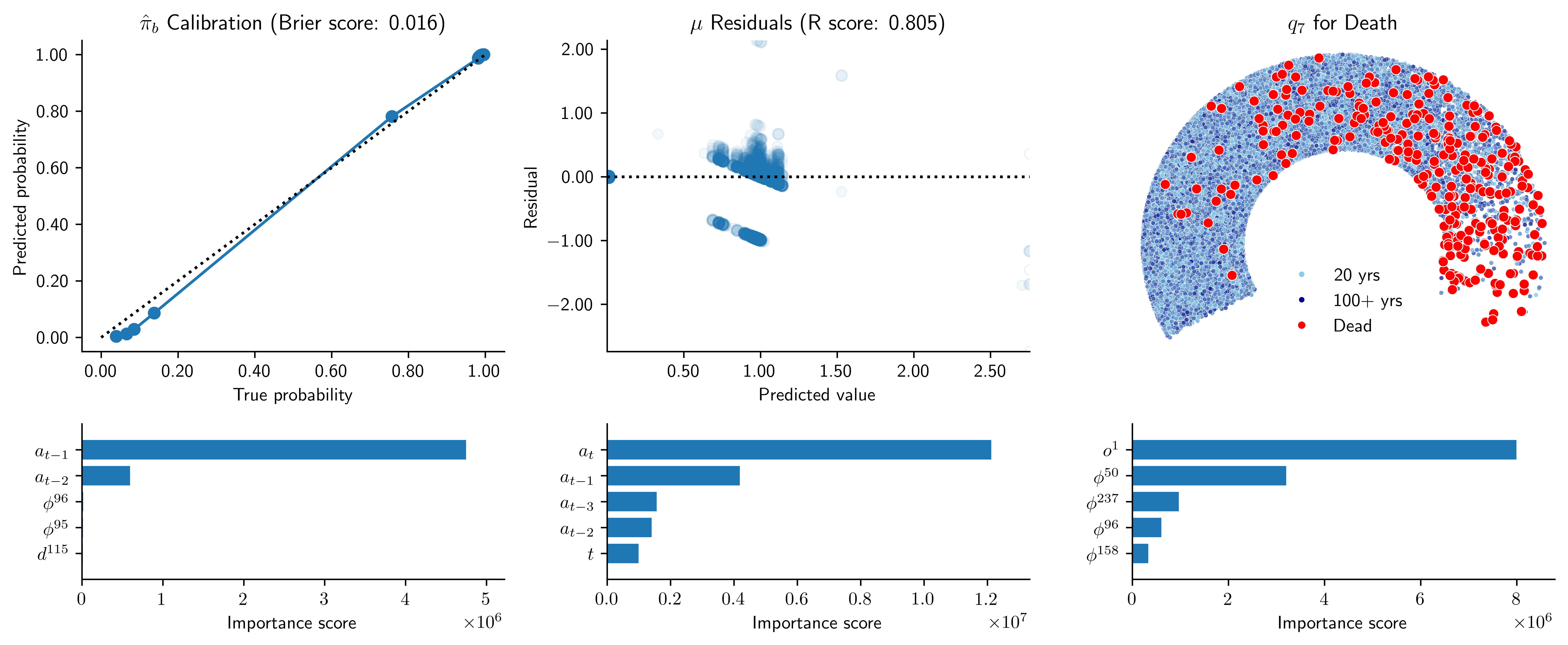
Out-of-fold diagnostics for the three nuisance functions. Left: \hat{\pi}_b calibration and \hat{\mu} residuals confirm reliable trajectory re-weighting. Top-right: rank-ordered \hat{q}_7 estimates — observed deaths (red) concentrate at the highest predicted-risk deciles, confirming mortality discrimination. Bottom: feature importance shows GPT history embeddings (\phi_t) are the primary predictors, secondary only to biological sex (\mathbf{o}^1).

OPE estimates:

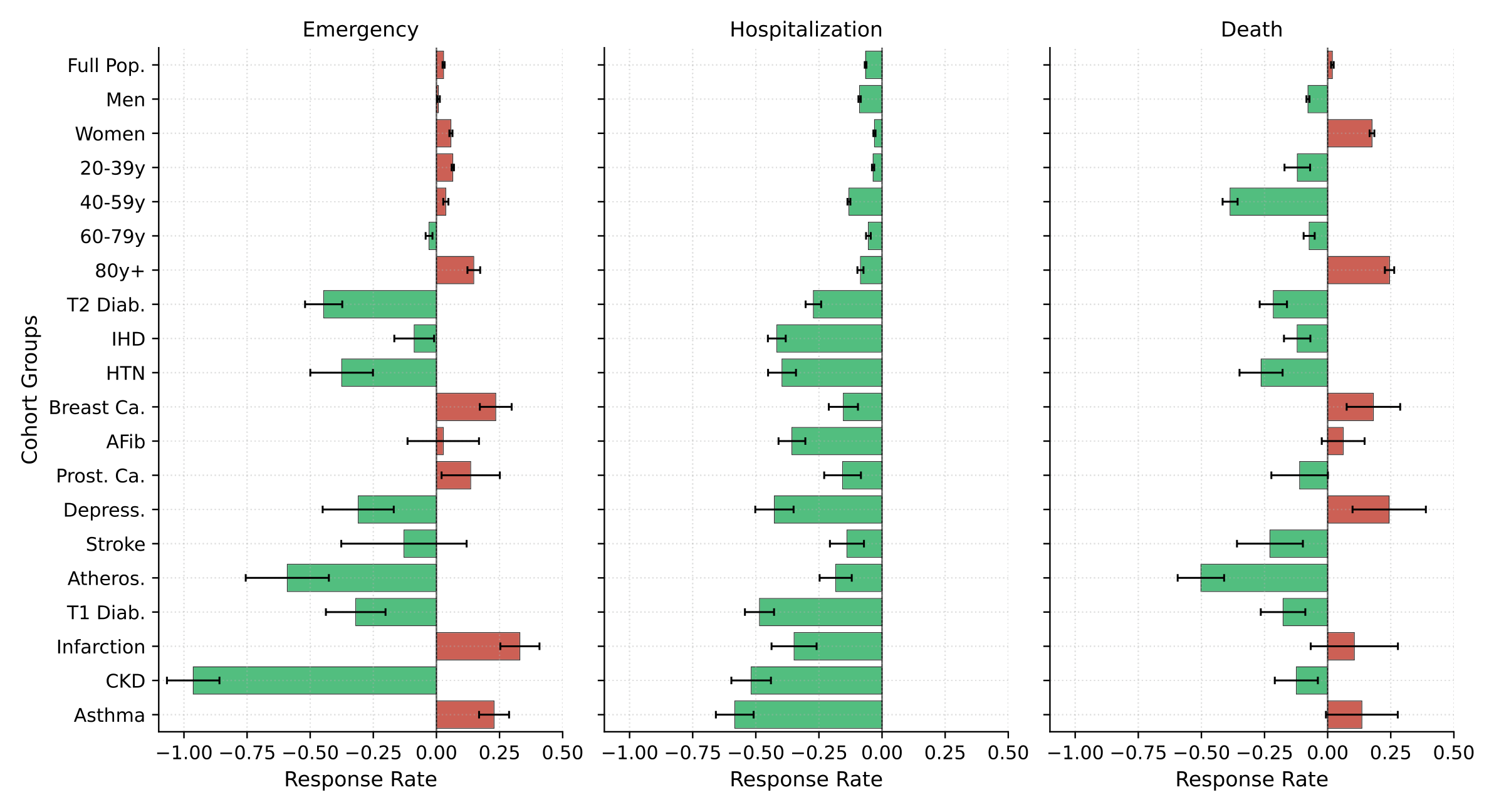
Doubly-robust OPE estimates of the G4H intervention effect across cohort subgroups and three outcomes (Emergency, Hospitalization, Death). Bars show the estimated response rate (95 % CI); green = beneficial reduction, red = adverse increase.

4 Avenues of work

Future work

• Other OPE use cases
  • HAS recommendations
  • Other rewards: total expenditures…
• Other GPT for medical pathways use cases:
  • causal inference
  • generation of synthetic trajectories
• Improve the foundation model:
  • Benchmarks
  • Make the embeddings really Markovian…

References

Chernozhukov, Victor, Denis Chetverikov, Mert Demirer, et al. 2018. Double/Debiased Machine Learning for Treatment and Structural Parameters. Oxford University Press Oxford, UK.

Kallus, Nathan, and Masatoshi Uehara. 2020. ‘Double Reinforcement Learning for Efficient Off-Policy Evaluation in Markov Decision Processes’. Journal of Machine Learning Research 21 (167): 1–63.

Shmatko, Artem, Alexander Wolfgang Jung, Kumar Gaurav, et al. 2025. ‘Learning the Natural History of Human Disease with Generative Transformers’. Nature, ahead of print, September 17. https://doi.org/10.1038/s41586-025-09529-3.

Waxler, Shane, Paul Blazek, Davis White, et al. 2025. Generative Medical Event Models Improve with Scale. arXiv:2508.12104. arXiv. https://doi.org/10.48550/arXiv.2508.12104.

Pres. link