SODA Seminar
Policy evaluation using Transformer-based medical pathway embeddings
31 March 2026
1 Introduction
About me
- Graduated from HEC (19-24), X (X20), ENSAE and MVA (administrateur de l’Insee, 2024)
- Internships:
- 2023: MIT (Operations Research Center), Microtransit system design and optimization
- 2024: Inria HeKA, Generative models for longitudinal images
- Currently, since sept. 2024:
- Data Scientist at Insee’s AI & Data Science Innovation Lab (MLOps, agentic workflows and deep learning use cases: NLP, ML/DL for econometrics, satellite imagery)
- PhD in CS Candidate (part-time) - supervised by G. Lecué (Crest) and G. Varoquaux (Inria)
Broader view of the Graph4Health ANR
- The general objective is to
- infer the impact of the healthcare supply (and its geographic distribution) on health outcomes
- using classic econometric tools
- using deep learning methods
- study policies that contribute to the efficiency of the French healthcare system
- infer the impact of the healthcare supply (and its geographic distribution) on health outcomes
- 11 years of exhaustive SNDS
- 70M patients
- consultations, procedures, hospitalizations, medications, deaths etc.
2 Transformer-based models for medical pathway embedding
Setting
Dataset of medical pathways: For i = 1, \dots, n, X_i \coloneqq (e_i, t_i, f_i), where:
- e_i \in \mathbb{R}^{cs} are the tokenized events, containing integers between 0 and the vocabulary size \lvert \mathcal{V} \rvert
- t_i \in \mathbb{R}^{cs} is the temporal vector, containing the dates
- f_i \in \mathbb{R}^{2} corresponds to the patient general features, for now age and gender
Tokenization
- Consultations: 83 tokens (specialties, e.g. general practitioner, cardiologist, etc.)
- Procedures: 936 tokens (CCAM codes)
- Medications: 704 tokens (ATC codes)
- Hospitalization entries: 3,275 tokens (ICD10 codes)
- Hospitalization exits: 1,110 tokens (DRG codes)
- Emergency entry: 1 token
- Death: 1 token
- Long-term disease (ALD): 1,110 tokens (ICD10 codes) + 1 token for “no long-term disease”
- Special tokens: [PAD], age, gender, “empty”…
These pathways are:
- unstructured (just as in NLP)
- temporally irregular (not like NLP!)
To feed downstream estimators, we need to represent those pathways as vectors (embeddings)
Objectives
- Having a time-aware Transformers (\neq NLP) with a lot of simultaneous events
- Need to design an adapted loss function
- Keeping in mind policy evaluation
- We want to be able to efficiently compute the embedding of the pathway at any time (the trajectory of the patient)
- Focus on decoder-only Transformers (GPT-like)
Model
- Embedding matrices of size \mathbb{R}^{\lvert \mathcal{V} \rvert, d_{embed}} (vocab), \mathbb{R}^{2, d_{embed}} (gender) and \mathbb{R}^{8, d_{embed}} (age class)
- We use t_i to have a time-aware positional encoding using a sinusoidal encoding
- A symbolic [START] token, composed of the summed embeddings of age and gender.
- Causal self-attention layers so that the Transformer-based model outputs causally contextualized embeddings: GPT_{\theta}(X_i) \in \mathbb{R}^{cs, d_{embed}}
Pre-training
- We use weight tying to output the logits \in \mathbb{R}^{cs, \lvert \mathcal{V} \rvert}
\text{logits}_{i, c, v} = (W \cdot GPT_{\theta}(X))_{i, c, v}
- Next-Token Prediction: instead of softmax as in Shmatko et al. (2025), we use a multi-label classification loss to better handle co-occurent events:
\text{BCE}_{i, c} \coloneqq - \sum_v y_{i, c, v} \log \frac{\lambda_{i, c, v}}{1 + \lambda_{i, c, v}} + (1-y_{i, c, v}) \log \frac{1}{1 + \lambda_{i, c, v}}
- Time-to-Next-Event Prediction: exactly as in Shmatko et al. (2025):
\text{TTE}_{i, c} \coloneqq - \log(\sum_v \lambda_{i, c, v}) + t^{*} \sum_v \lambda_{i, c, v}
Validating the model
Scaling law
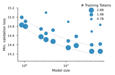
We are matching the ~2,000 optimal ratio \frac{\text{\# training tokens}}{\text{\# parameters}} found in Waxler et al. (2025).
Embedding space
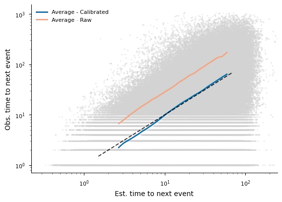
Time Calibration
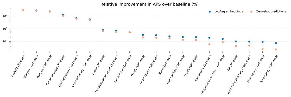
Predictive power
3 Off-Policy Evaluation
Markov Decision Processes and Off-Policy Evaluation
- A Markov Decision Process (MDP) is a tuple (\mathcal{S}, \mathcal{A}, P, P_0, R, \gamma) where:
- \mathcal{S} is the state space
- \mathcal{A} is the action space
- P: \mathcal{S} \times \mathcal{A} \to \Delta(\mathcal{S}) is the transition probability function
- P_0 \in \Delta(\mathcal{S}) is the initial state distribution
- R: \mathcal{S} \times \mathcal{A} \to \mathbb{R} is the reward function
- \gamma \in [0,1] is the discount factor
A policy \pi: \mathcal{S} \to \Delta(\mathcal{A}) is a mapping from states to distributions over actions (\pi(a|s) is the probability of taking action a in state s under policy \pi).
A T-step trajectory \tau generated by policy \pi is a sequence of states, actions and rewards: \tau \coloneqq (s_0^i, a_0^i, r_0^i \dots s_{T-1}^i, a_{T-1}^i, r_{T-1}^i, s_T^i) where:
- s_0^i \sim P_0 is the initial state
- a_t^i \sim \pi(\cdot | s_t^i) is the action taken at time t
- s_{t+1}^i \sim P(\cdot | s_t^i, a_t^i) is the next state
- r_t^i = R(s_t^i, a_t^i) is the reward received at time t
The return of a trajectory \tau is the discounted sum of rewards: G(\tau) = \sum_{t=0}^{T-1} \gamma^t r_t^i.
We are interested in the value of a policy \pi, defined as the expected return of trajectories generated by \pi: V^{\pi} = \mathbb{E}_{\tau \sim P^{\pi}}[G(\tau)] where P^{\pi}(\tau) is the distribution of trajectories generated by policy \pi.
- The Off-Policy Evaluation (OPE) problem assumes:
- We have access to a dataset of T-step trajectories \mathcal{D} = \{\tau^i\}_{i=1}^N generated by an unknown behavioral policy \pi_b: \mathcal{S} \to \Delta(\mathcal{A}).
- We want to estimate the value V^{\pi_e} of a target policy \pi_e: \mathcal{S} \to \Delta(\mathcal{A}) using only the dataset \mathcal{D}.
- Step-Weighted Importance Sampling estimator: \hat{\rho}_{\mathrm{step}-\mathrm{WIS}}^{\pi_e}=\sum_{i=1}^n \sum_{t=0}^{T-1} \gamma^t \frac{\omega_{0: t}^{i} r_t^{i}}{\sum_{i=1}^n \omega_{0: t}^{i}} where \omega_{0: t}^{i}=\prod_{t'=0}^t \frac{\pi_e(a_{t'}^{i} | s_{t'}^{i})}{\hat{\pi}_b(a_{t'}^{i} | s_{t'}^{i})} is the importance weight of trajectory i up to time t.
See Farajtabar et al. (2018) for more details on OPE estimators and their properties.
In our case
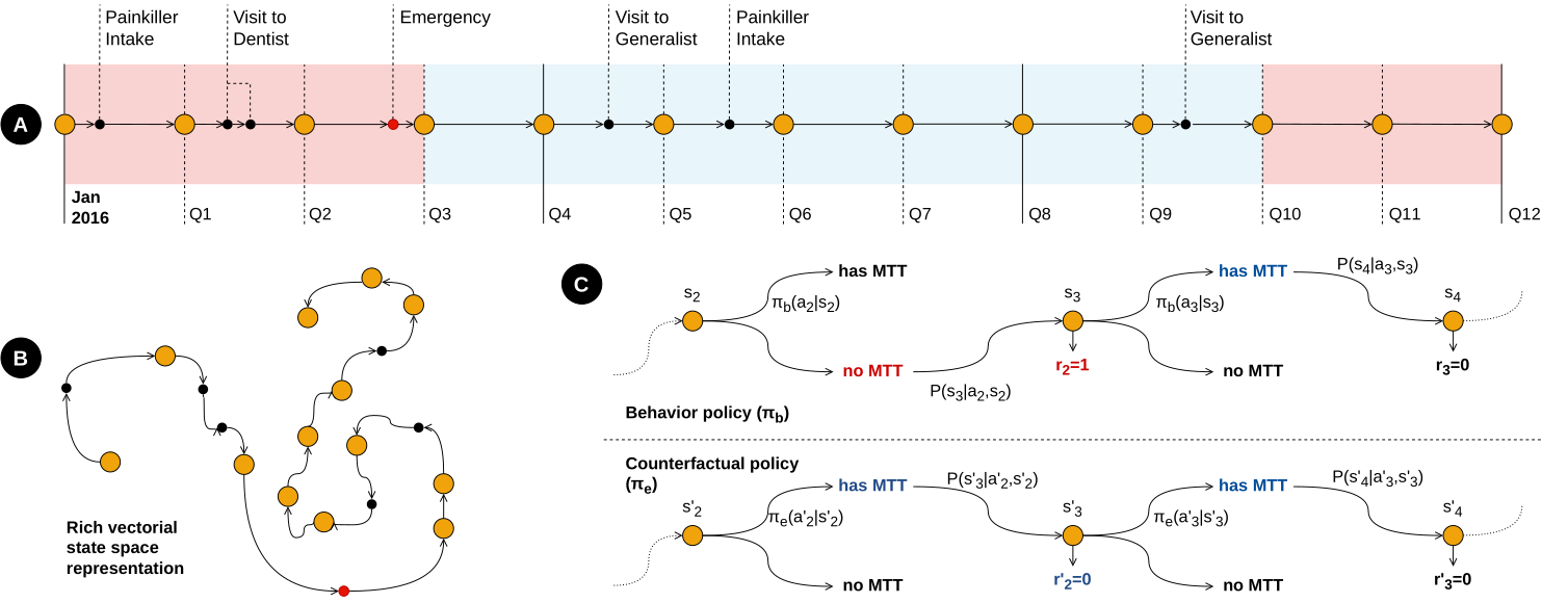
- Reinforcement learning framework
- State: embedding of the patient at the end of each quarter
- Sufficient statistic that summarizes the patient’s history
- Markov assumption: the future only depends on the current state
- Action: whether the patient has a PCP or not at the beginning of next quarter
- Reward: number of emergency visits within the next quarter (or hospitalization entries)
- State: embedding of the patient at the end of each quarter
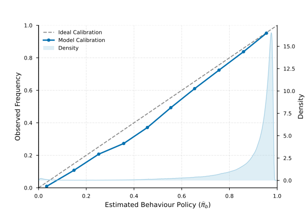
Estimation of the behavioral policy
First step of the OPE pipeline: regress a_{i,t} (PCP affiliation) on s_{i,t} (embeddings) to estimate \hat{\pi}_b(a|s), the behavioral policy.
V^{\pi_b} and \pi_e
The value of the behavioral policy can be estimated using the trajectories in the dataset \mathcal{D}:
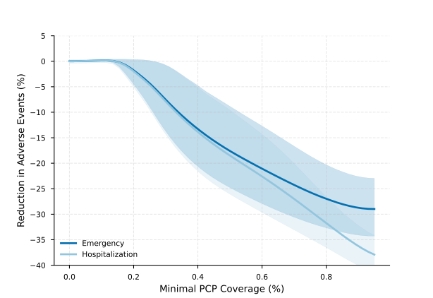
V^{\pi_b} \approx V^{\hat{\pi}_b} \coloneqq \frac{1}{N} \sum_{i=1}^N \sum_{t=0}^{T-1} \gamma^t r_t^iThe policies we want to study: \pi_e^\eta(1|s) = \max(\eta, \hat{\pi}_b(1|s)) for \eta = 0 \dots 0.99
Results
General population
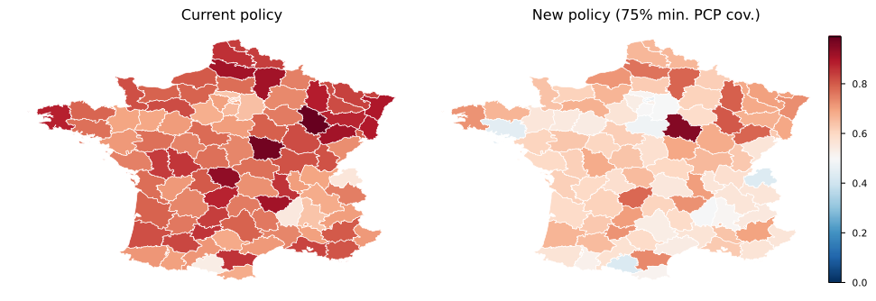
Geographical heterogeneity
| Subpopulation | Emergency (%) | Hospit. (%) | Size | PCP |
|---|---|---|---|---|
| General Population | (31.8–18.8) | (35.0–23.7) | 10.39 | 87.4% |
| Age Group | ||||
| 20–29 | (25.1–22.5) | (29.3–16.1) | 1.38 | 72.9% |
| 30–39 | (1.1)–0.1 | (0.5)–3.0 | 1.65 | 84.6% |
| 40–49 | 0.4–1.5 | 2.0–7.9 | 1.65 | 88.4% |
| 50–59 | (4.9)–1.3 | (4.7)–3.0 | 1.70 | 91.2% |
| 60–69 | (18.5–7.7) | (20.0–8.3) | 1.55 | 92.7% |
| 70–79 | (16.3–6.6) | (17.5–7.9) | 1.26 | 93.8% |
| 80–89 | (37.9–17.1) | (37.6–18.6) | 0.76 | 92.1% |
| 90+ | (18.5–14.2) | (19.3–15.2) | 0.39 | 82.7% |
| Sex | ||||
| Male | (19.3–17.0) | (24.2–21.6) | 5.00 | 85.2% |
| Female | (33.1–19.5) | (35.3–24.4) | 5.38 | 89.5% |
| Subpopulation | Emergency (%) | Hospit. (%) | Size | PCP |
|---|---|---|---|---|
| General Population | (31.8–18.8) | (35.0–23.7) | 10.39 | 87.4% |
| Clinical (ALD) | ||||
| Type 2 diabetes | (30.5–21.2) | (34.0–25.5) | 0.59 | 87.4% |
| Primary hypertension | (32.9–17.3) | (36.2–21.5) | 0.16 | 87.4% |
| Mal. neoplasm of breast | (17.2–9.6) | (21.9–13.9) | 0.18 | 87.4% |
| Mal. neoplasm of prostate | (25.2–5.1) | (28.5–14.7) | 0.12 | 87.4% |
| Depressive episodes | (18.7–4.3) | (25.6–16.9) | 0.11 | 87.6% |
| Stroke | (15.2–3.7) | (23.7–15.1) | 0.09 | 87.4% |
| Dementia in Alzheimer | (20.1–7.8) | (25.6–14.0) | 0.08 | 87.4% |
| Heart failure | (15.2)–1.9 | (24.4–13.2) | 0.08 | 87.4% |
4 Avenues of work
Future work
- Other actions
- HAS recommendations
- Other rewards
- Total expenditures…
- Apply the method to specific subpopulations
- Diabetes
- Heart failure
- Enriching the embedding
- Smarter training losses
- Action as token