From Accuracy to Trust
Practical Methods for Uncertainty-Aware Automatic Coding with ML and xAI
Institut national de la statistique et des études économiques (INSEE)
2026-05-12
Agenda
- The accuracy illusion — why 95% is not enough
- Pillar I — measuring what matters: calibration & risk-coverage
- Pillar II — building for uncertainty: multi-level heads & label attention
- Practical take-aways
The Accuracy Illusion
A model that is right 95% of the time
The setting
A deep learning model automatically codes job descriptions into ISCO-08 occupations if confidence is high enough, otherwise it is sent to manual annotation.
- Training accuracy: 95.3 %
- Test accuracy: 94.8 %
- Sounds production-ready.
The reality — at INSEE’s scale
| Volume | Errors |
|---|---|
| 100 000 records / year | 5 200 wrong codes |
| Sent automatically, unreviewed | all 5 200 |
| Statistician detects the pattern | months later |
The model does not know when it is wrong. A confident wrong prediction is the worst failure mode in official statistics.
Two very different 5 % errors
Model A — confused but honest
Predicts Nurse with probability 0.52 when the true code is Midwife.
→ A threshold of 0.7 catches this. → The record goes to a human reviewer. → No damage done.
Model B — confident and wrong
Predicts Software developer with probability 0.97 when the true code is Data entry clerk.
→ No threshold catches this. → Published automatically. → Systematic bias in employment statistics.
Accuracy measures how often we are right. It says nothing about when we know we are right. That gap is what we need to close.
Pillar I — The Right Metrics
What we actually need from a probability
A classifier outputs P(class | text). We want this number to mean something:
Among all predictions made with confidence 80 %, exactly 80 % should be correct.
This property is called calibration. A well-calibrated model turns confidence into a reliable operational signal.
Calibration ≠ Accuracy. A model can be highly accurate yet badly miscalibrated — and vice-versa. Modern deep learning tends to be overconfident.
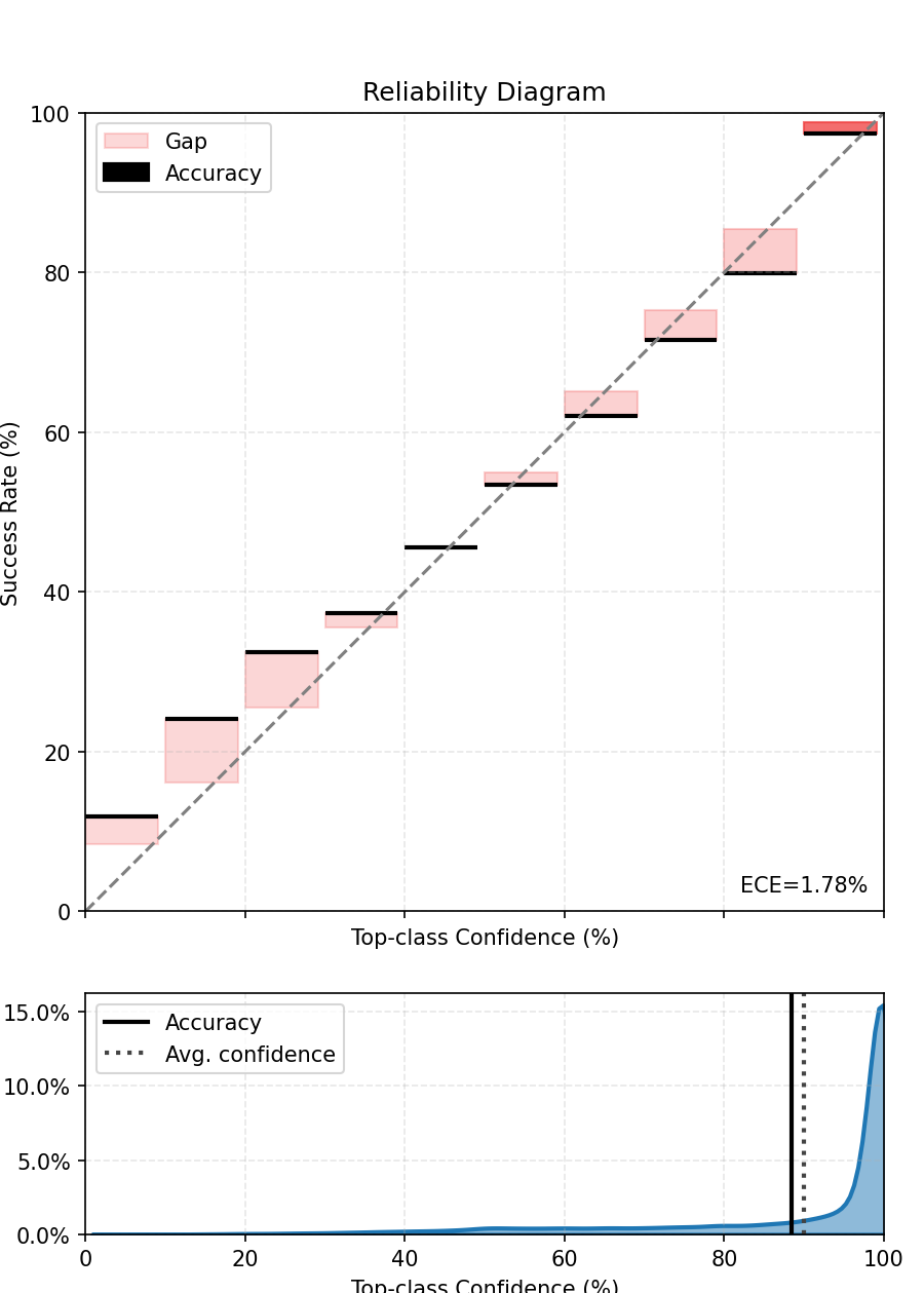
The reliability diagram
- Perfect calibration: actual accuracy = predicted confidence (diagonal line)
- Overconfident model: bars above the diagonal — the model is more sure than it should be
- ECE (Expected Calibration Error): average gap between confidence and accuracy, weighted by bin size — one number to compare models
ECE gives a single diagnostic number. A well-calibrated model has ECE close to 0. Post-hoc techniques (temperature scaling, isotonic regression) can correct miscalibration without retraining.
For models based on PyTorch, the torch-uncertainty package offer several ready-to-use modules.
From calibration to decisions: risk–coverage curves
Set a confidence threshold τ: above τ → automate · below τ → human review
Coverage = share of records automated
Risk = error rate among automated records
These two quantities move in opposite directions as τ varies.
The risk–coverage curve answers: “If we accept a 1 % error rate, what share of our volume can we automate?” — a question accuracy cannot answer.

Comparing models with risk–coverage curves
A model that dominates another sits lower and to the right on the curve — lower risk for the same coverage.
Key operational question: where is your institutional risk tolerance?
- Set a maximum acceptable error rate (e.g. 0.5 %)
- Read off the maximum achievable automation rate
- Compare models at that operating point — not on accuracy alone
Practical workflow: train → calibrate → plot risk-coverage → choose τ consistent with your quality constraints → monitor stability after deployment.
Pillar II — The Right Architecture
Hierarchical classifications demand hierarchical models
ISCO, NACE, CPA — all share the same structure: a tree.
- Level 1 (Major groups): 10 categories — easy
- Level 2 (Sub-major groups): 43 categories — moderate
- Level 3 (Minor groups): 130 categories — hard
- Level 4 (Unit groups): 436 categories — very hard
Standard approach: one softmax head at the finest level.
The problem: when the model is uncertain at level 4, it often already knows the right level-2 code. Forcing a fine-grained wrong answer wastes that signal.
Insight: uncertainty should trigger a graceful degradation to a coarser but correct code — not a confident wrong fine code.
Multi-level prediction heads
Architecture
One shared encoder → One prediction head per level of the hierarchy
At inference time:
- Check confidence at level 4
- If below τ₄, fall back to level 3 head
- If below τ₃, fall back to level 2 head
- …
Benefits
- Partial automation: fine codes where confident, coarser codes otherwise
- Limits catastrophic errors (wrong fine code that contradicts the right major group)
- “Smarter” models that understand the full hierarchy of the classification
The fallback mechanism transforms uncertainty from an obstacle into a feature: we always give the most precise answer we can trust.
Label attention: towards xAI
Label attention: each ISCO code gets its own embedding vector (learned matrix of size \(n_{labels} \times d_{embed}\)). A cross-attention layer uses label embeddings as queries and token embeddings as keys/values, producing one label-conditioned sequence embedding per ISCO code, each scored by a linear probe.
Why it helps
- The model learns what discriminates codes, not just which index wins -> better performance and calibration
- Attention weights are directly interpretable: how much a token is driving the prediction ?
- Useful for human reviewers in production


Putting the two pillars together
Pillar I — Right metrics
- Reliability diagram + ECE: diagnose calibration
- Post-hoc calibration: fix it without retraining
- Risk-coverage curve: choose your operating point
- Monitor drift: re-check after each production cycle
Pillar II — Right architecture
- Multi-level heads: graceful degradation under uncertainty
- Label attention: richer representations + explainability
- All those are available in the torchTextClassifiers, a toolkit to easily train and deploy a text classification PyTorch-based deep learning model!
The combination: an architecture that knows what it knows, metrics that reveal when it doesn’t, and curves that let managers set the acceptable risk — before going live, not after the damage is done.
Take-Aways
What to bring back to your NSI
Do not deploy on accuracy alone.
| Question | Tool |
|---|---|
| Are my probabilities meaningful? | Reliability diagram + ECE |
| Can I fix miscalibration cheaply? | Temperature scaling / isotonic regression |
| What automation rate can I afford? | Risk-coverage curve at your risk tolerance |
| How to handle hierarchical codes? | Multi-level heads + confidence fallback |
| How to explain a prediction to a reviewer? | Label attention + Layer Integrated Gradients |
| How to monitor after deployment? | Track ECE drift + risk-coverage stability |
The goal is to automate confidently what the model knows, and flag honestly what it does not.
Thank You

![]()